Yapay Zeka Destekli Trading Stratejileri: Makine Öğrenmesi ile Algoritmik Ticaret
Makine öğrenmesi ve derin öğrenme kullanarak profesyonel trading stratejileri geliştirme. Feature engineering, LSTM modelleri ve piyasa duygu analizi.
Giriş: Finansal Piyasalarda Paradigma Değişimi
Geleneksel teknik analiz yöntemleri (RSI, MACD gibi indikatörler), geçmiş fiyat hareketlerinin gelecekte tekrarlanacağı varsayımına dayanır. Ancak modern piyasalar, yüksek frekanslı işlemler (HFT) ve kurumsal algoritmaların hakimiyeti altındadır. Bir senior mühendis için “Yapay Zeka Destekli Trading”, sadece basit bir model eğitmek değil; veri toplama, temizleme, feature engineering ve risk yönetimi süreçlerini kapsayan uçtan uca bir mühendislik disiplinidir.
Bu rehberde, ham piyasa verisini nasıl anlamlı sinyallere dönüştüreceğimizi, derin öğrenme (LSTM) ve ensemble (Random Forest) metotlarının avantajlarını ve prodüksiyon seviyesinde karşılaşılan zorlukları ele alacağız.
Strateji Mimarisi: Veriden Sinyale Giden Yol
Başarılı bir AI trading sistemi dört temel katmandan oluşur:
1. Veri Ingestion ve Temizleme
Sadece OHLCV (Open, High, Low, Close, Volume) verisi yeterli değildir. Orderbook derinliği, on-chain veriler (kripto için) ve makroekonomik veriler sisteme dahil edilmelidir.
- Problem: Kirli veri (outliers, missing values).
- Çözüm: Z-score normalizasyonu ve lineer interpolasyon teknikleri.
2. Feature Engineering: Sinyal Gücünü Artırma
Modelin başarısı, modelin kendisinden çok ona verdiğiniz özelliklere (features) bağlıdır. Teknik indikatörlerin ötesinde “volatility clustering” ve “fourier transforms” gibi ileri matematiksel özellikler eklemek, gürültüyü (noise) azaltır.
3. Model Eğitimi ve Seçimi
- Sınıflandırma (Classification): Fiyatın çıkacağını (1), düşeceğini (-1) veya yatay kalacağını (0) tahmin eder.
- Regresyon (Regression): Fiyatın tam olarak ne kadar değişeceğini (yüzdesel) tahmin eder.
Feature Engineering: Ham Veriden Anlam Çıkarmak
Bir senior analist olarak, ham fiyat verisini direkt modele vermekten kaçınmalısınız. Modeller, fiyatın kendisinden ziyade “fiyat değişim oranları” (pct_change) ve “volatilite” (Standard Deviation) ile daha iyi öğrenir.
1
2
3
4
5
6
7
8
9
10
11
12
import pandas_ta as ta

def enhance_data(df):
    # Trend ve Momentum
    df['RSI'] = ta.rsi(df['close'], length=14)
    df['MACD'] = ta.macd(df['close'])['MACD_12_26_9']

    # Volatilite ve Likidite
    df['ATR'] = ta.atr(df['high'], df['low'], df['close'], length=14)
    df['Volume_Ratio'] = df['volume'] / df['volume'].rolling(20).mean()

    return df.dropna()
Feature selection sürecinde, birbirine aşırı korelasyonu olan indikatörleri (örneğin SMA_20 ve EMA_20) ayıklamak, modelin “overfitting” (aşırı öğrenme) riskini azaltır.
Derin Öğrenme: LSTM ile Zaman Serisi Tahmini
Zaman serisi verileri (fiyatlar), sıradan sinir ağları tarafından işlenirken veri noktaları arasındaki zamansal ilişki kaybolur. LSTM (Long Short-Term Memory) ağları ise, geçmişteki önemli olayları “hatırlama” ve alakasız gürültüleri “unutma” yeteneğine sahiptir.
Senior Notu: LSTM modelleri çok fazla hiperparametre (lookback period, hidden layers, dropout rate) gerektirir. Lookback süresini çok uzun tutmak “lag” (gecikme) oluştururken, çok kısa tutmak önemli trendleri kaçırmanıza neden olur.
1
2
3
4
5
6
7
8
9
10
11
12
13
from tensorflow.keras.models import Sequential
from tensorflow.keras.layers import LSTM, Dense, Dropout

def build_model(input_shape):
    model = Sequential([
        LSTM(units=50, return_sequences=True, input_shape=input_shape),
        Dropout(0.2),
        LSTM(units=50, return_sequences=False),
        Dropout(0.2),
        Dense(units=1, activation='linear')
    ])
    model.compile(optimizer='adam', loss='mean_squared_error')
    return model
Sentiment Analizi: Sosyal Medyanın Nabzını Tutmak
Özellikle kripto para piyasalarında fiyatı sadece grafikler değil, “hype” (popülerlik) ve “fud” (korku) belirler. Twitter ve Reddit verilerinden çekilen duygu skorları, modelin başarısını ciddi oranda artırabilir.
NLP ile Duygu Skorlama:
Modelin içine Sentiment_Score adında bir feature ekleyerek, o günkü haberlerin veya tweetlerin ne kadar pozitif/negatif olduğunu belirtebiliriz.
- Teknik: BERT veya VADER gibi kütüphanelerle metinlerin “Polarity” ve “Subjectivity” değerlerini hesaplayıp sisteme beslemek.
Ensemble Yöntemleri: Random Forest ve Feature Importance
Derin öğrenme modelleri “black box” (kara kutu) gibi çalışırken, Random Forest gibi ağaç tabanlı modeller bize hangi verinin daha önemli olduğunu söyler. feature_importances_ özniteliği sayesinde, stratejinizde RSI’ın mı yoksa İşlem Hacmi’nin mi daha belirleyici olduğunu görebilirsiniz.
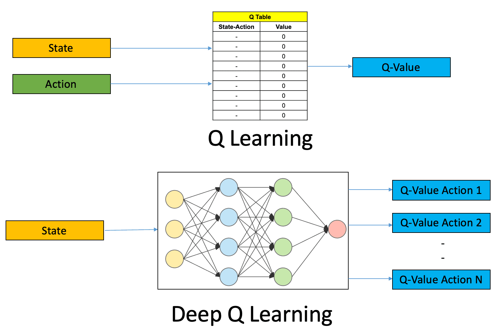
Reinforcement Learning (Takviyeli Öğrenme): Geleceğin Vizyonu
Geleneksel modeller sadece “tahmin” yaparken, Reinforcement Learning (RL) “aksiyon” (al, sat, tut) almayı öğrenir. Model, başarılı işlemlerden ödül (reward), başarısız işlemlerden ceza alarak zamanla en karlı stratejiyi kendi başına geliştirir.
Backtesting: Hayaller ve Gerçekler
Modeliniz eğitim setinde (train set) %90 doğruluk veriyor olabilir ama bu, gerçek piyasada para kazanacağı anlamına gelmez. Bir senior mühendisin en büyük düşmanı “overfitting”dir.
Walk-Forward Validation (İleriye Dönük Doğrulama)
Statik bir train-test split yerine, zaman penceresini kaydırarak (sliding window) test yapmak çok daha sağlıklı sonuçlar verir. Bu yöntem, modelin piyasa rejim değişikliklerine (bullish vs bearish) nasıl tepki verdiğini ölçer.
1
2
3
4
5
6
import vectorbt as vbt

# Basit bir backtest örneği
signals = model.predict(X_test) > 0.6 # %60 üzeri güvenle al
portfolio = vbt.Portfolio.from_signals(close_prices, signals)
portfolio.plot().show()
Dikkat: “Backtest overfitting” makale yazmak için harikadır ama portföyünüzü sıfırlayabilir. Hatalı komisyon oranları ve “slippage” (kayma) maliyetlerini hesaba katmayı unutmamalısınız.
Risk Yönetimi: Modeli Korumak
Hiçbir model %100 başarılı olamaz. Başarının anahtarı, hatalı tahminler yapıldığında sermayeyi korumaktır.
- Stop-Loss (Zarar Kes): Model her ne kadar “al” dese de, fiyat belirli bir oranın altına indiğinde işlemi otomatik kapatmak.
- Kelly Criterion (Pozisyon Büyüklüğü): Kazanç ihtimaline göre ne kadar sermaye ile işleme girileceğini dinamik olarak belirlemek.
- Drawdown Kontrolü: Toplam portföy kaybı belirli bir eşiği geçerse algoritmayı pasif moda çekmek.
Senior Hataları: Look-ahead Bias ve Data Leakage
Yeni başlayanların en çok düştüğü iki dev hata vardır:
1. Data Leakage (Veri Sızıntısı)
Modele yanlışlıkla “gelecekten” bilgi vermektir. Örneğin, bugünkü volatiliteyi hesaplarken yarının fiyatını da hesaba katarsanız, modeliniz kağıt üzerinde kusursuz çalışır ama gerçekte imkansızdır.
2. Look-ahead Bias
İşlem yapma zamanı ile verinin kullanılabilir olduğu zaman arasındaki farkı kaçırmak. Örneğin, saat 12:00 mumu kapandığında, o mumun verisi ancak 12:00:01’de işlenebilir. Eğer 12:00’deki kapanış fiyatından hemen o saniyede işlem açtığınızı varsayarsanız, hayali bir performans elde edersiniz.
Production ve Monitoring: Modeli Canlıya Almak
Modeli başarıyla eğitmek işin sadece yarısıdır. Gerçek dünyada modelin performansını sürdürebilmesi için sürekli izleme (monitoring) gerekir.
- Düşük Latency (Gecikme): Modelinizin tahmin üretme süresi, piyasanın hareket hızından yavaş olmamalıdır.
- Concept Drift (Kavram Kayması): Piyasa koşulları zamanla değişir (volatilite artışı, yeni oyuncular). Modelin doğruluğu düştüğünde otomatik olarak yeniden eğitilmesi (re-training) planlanmalıdır.
- Hata Takibi: API kesintileri veya beklenmedik piyasa hareketlerinde algoritmanın nasıl davranacağı önceden kodlanmalıdır. “Circuit breaker” (devre kesici) mantığı, ekstrem durumlarda büyük kayıpları engeller.
Teknik Sözlük (Glossary)
- LSTM (Long Short-Term Memory): Zaman serisi verilerinde uzun vadeli bağlantıları öğrenebilen özel bir sinir ağı türü.
- Feature Engineering: Ham veriyi makine öğrenmesi modelleri için daha anlamlı özelliklere dönüştürme süreci.
- Overfitting: Modelin eğitim verilerine aşırı uyum sağlayıp, yeni verilere karşı başarısız olması.
- Backtesting: Bir stratejinin geçmiş veriler üzerinde ne kadar başarılı olduğunu test etme işlemi.
- Sentiment Analysis: Metin tabanlı verilerden (haber, tweet) toplumsal duygu ve görüşlerin analiz edilmesi.
- Sharpe Ratio: Bir yatırımın aldığı riske göre sunduğu getiriyi ölçen bir finansal rasyo.
- Slippage: İşlemin niyet edilen fiyattan farklı bir fiyatta gerçekleşmesi durumu.
- Data Leakage: Gelecekten gelen bilgilerin yanlışlıkla modelin eğitim sürecine girmesi.
Sonuç: Yapay Zeka ile Finansal Özgürlük Mümkün mü?
Yapay zeka, finans dünyasında kuralları yeniden yazsa da sihirli bir değnek değildir. Başarı; titiz bir mühendislik çalışması, sürekli veri analizi ve disiplinli risk yönetiminden geçer. Kendi AI trading sisteminizi kurmak istiyorsanız, önce küçük veri setleriyle başlamalı ve modellerinizin neden hatalı kararlar verdiğini anlamaya çalışmalısınız.
Eğer bu verileri gerçek zamanlı bir bot haline getirmek isterseniz Python ile Binance WebSocket Trading Bot rehberimizi okuyabilir, blockchain verilerini doğrudan çekmek için de Web3.py ile Ethereum Etkileşimi yazımıza göz atabilirsiniz.
Yapay zeka yolculuğunuzda en büyük sermayeniz veriniz, en büyük koruyucunuz ise kurduğunuz risk yönetimi sistemi olacaktır.