Pandas Optimize Edilmezse Python Yavaştır: Kripto Para Analizi Örneği

Python “yavaş” bir dildir, bu bir sır değil. Ancak Pandas performans sorunları genellikle dilin kendisinden değil, araçların yanlış kullanımından kaynaklanır. Veri biliminde “Analizim saatler sürüyor” şikayetinin arkasında genelde Pandas içine gömülmüş Python döngüleri yatar. Bu yazıda, gerçek bir Kripto Para Piyasası verisi (OHLCV) üzerinden, Pandas kodunuzu nasıl 100 kat hızlandırabileceğinizi anlatacağım.

Vektörizasyonun gücü: Saniyeler vs Dakikalar.

1. Düşmanımızı Tanıyalım: iterrows() ve apply()

Pandas’a yeni başlayanların (ve hatta bazı orta seviye geliştiricilerin) en büyük alışkanlığı, DataFrame üzerinde satır satır gezmektir. “Her satırın kapanış fiyatını al, açılış fiyatından çıkar, farkı yeni sütuna yaz”.

Yanlış Yöntem (Python Döngüsü - iterrows):

import pandas as pd
df = pd.read_csv("bitcoin_hourly.csv")

# YÖNTEM 1: iterrows() - AŞIRI YAVAŞ
diffs = []
for index, row in df.iterrows():
    diffs.append(row['close'] - row['open'])
df['diff_loop'] = diffs

Bu kod, her satır için bir Series objesi oluşturduğundan milyonlarca satırda dakikalar sürer.

Yarı Yanlış Yöntem (apply):

# YÖNTEM 2: apply() - YAVAŞ (Hala döngü var)
df['diff_apply'] = df.apply(lambda row: row['close'] - row['open'], axis=1)

apply vektörize değildir, satır bazlı çalışır. Native vektörizasyon her zaman daha iyidir.

2. Kurtarıcımız: Vectorization (Broadcasting)

Pandas ve NumPy, “SIMD” (Single Instruction, Multiple Data) mantığıyla çalışır. İşlemciye “Bu 1 milyon sayıyı al, şu 1 milyon sayıdan çıkar” talimatını tek seferde verir. Python döngüsü (loop) yoktur, her şey C seviyesinde biter.

Doğru Yöntem (Vektörizasyon):

# YÖNTEM 3: Vektörizasyon - IŞIK HIZI
# Pandas bütün sütunu tek bir NumPy dizisi (array) gibi görür.
df['diff_vector'] = df['close'] - df['open']

Bu kod iterrows’a göre 1000 kat daha hızlı çalışabilir. Kodunuzda for veya apply görüyorsanız, durup düşünün: “Bunu vektörize edebilir miyim?”

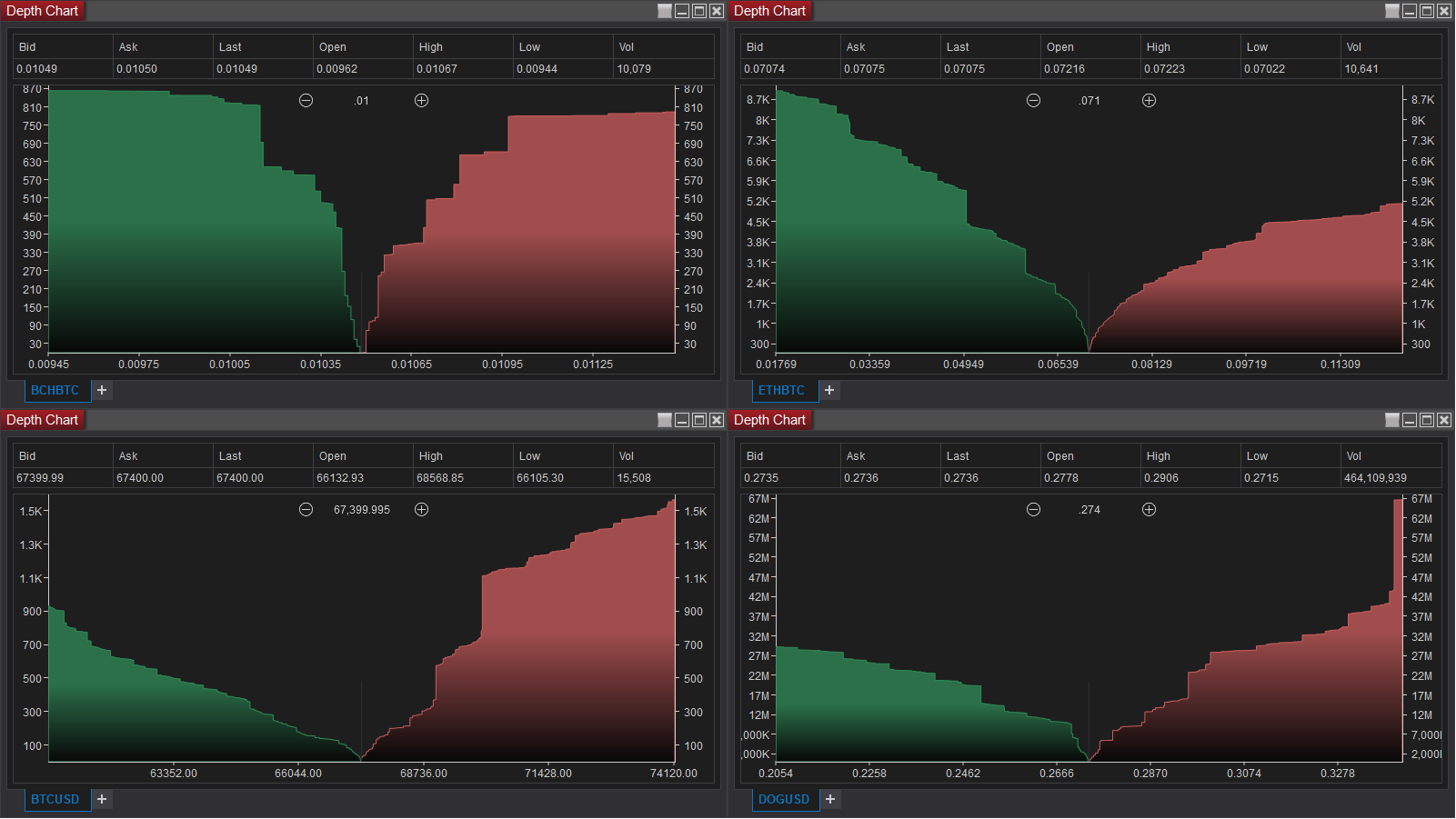
3. Gerçek Dünya Senaryosu: Hareketli Ortalamalar ve Sinyaller

Kripto para trade botu yazdığınızı düşünün. 50 saatlik ve 200 saatlik hareketli ortalamaları (MA) hesaplayıp, “Golden Cross” (Kesişim) olduğu anları bulacağız.

# Hatalı/Yavaş Yaklaşım: Döngü ile MA hesaplama
# SAKIN YAPMAYIN!
# for i in range(50, len(df)): ...

# Doğru Yaklaşım: rolling() penceresi
df['MA50'] = df['close'].rolling(window=50).mean()
df['MA200'] = df['close'].rolling(window=200).mean()

# Sinyal Üretimi (Condition Vectorization)
import numpy as np

# np.where, Excel'deki IF formülü gibidir ama tüm tabloya aynı anda uygulanır
# MA50 > MA200 ise BUY, değilse SELL
df['signal'] = np.where(df['MA50'] > df['MA200'], 'BUY', 'SELL')

Gördüğünüz gibi, hiç döngü yok. 10 yıllık Bitcoin verisini (dakikalık veri olsa bile), bu kodla saniyeler içinde işleyebilirsiniz. Pandas’ın rolling, expanding, shift gibi fonksiyonları, zaman serisi analizleri için optimize edilmiştir. Örneğin bugünün kapanışını dünkü kapanışla kıyaslayacaksanız: df['daily_return'] = df['close'] / df['close'].shift(1) - 1 Bu kadar basit.

OHLCV verileri üzerinde hareketli ortalamalar ve trend analizi.

4. Bellek Yönetimi: “MemoryError” Kabusu

Pandas varsayılan olarak sayıları int64 veya float64, metinleri ise object olarak tutar. Ancak çoğu zaman bu kadar hassaslığa ihtiyacınız yoktur. Kripto para hacmi için 64 bit integer gerçekten gerekli mi?

• Fiyat verisi için float32 yeterlidir.
• Hacim (Volume) verisi için int32 yeterlidir.
• Kategorik veriler (“BUY”, “SELL”, “BTC/USDT”) için category tipi kullanılmalıdır.

# RAM kullanımını %70 azaltan basit tip dönüşümleri
df['volume'] = df['volume'].astype('int32')
df['close'] = df['close'].astype('float32')
df['signal'] = df['signal'].astype('category')

String sütunlarını category tipine çevirmek (eğer tekrar eden değerler varsa), bellekte metin yerine integer pointer tutulmasını sağlar. Bu da işlem hızını ve bellek verimliliğini inanılmaz artırır. Büyük veri (Big Data) ile çalışıyorsanız, CSV okurken pd.read_csv(..., dtype={'volume': 'int32'}) diyerek daha baştan tasarruf edebilirsiniz.

5. Zincirleme İşlemler (Method Chaining)

Modern Pandas kodu, adım adım değişken atamak yerine, akıcı (fluent) bir zincirleme stilini benimser. R dilindeki dplyr‘a benzer. Bu kodun okunabilirliğini artırır ve ara değişkenlerin belleği kirletmesini önler.

# Eski Tarz
df1 = df.dropna()
df2 = df1[df1['volume'] > 1000]
df3 = df2.assign(price_range = df2['high'] - df2['low'])

# Modern Tarz (Method Chaining)
result = (
    df
    .dropna()
    .query("volume > 1000")
    .assign(price_range=lambda x: x['high'] - x['low'])
    .sort_values("date")
    .reset_index(drop=True)
)

Debugging yaparken araya .pipe(print_shape) gibi kendi fonksiyonlarınızı ekleyebilirsiniz. Bu stil, kodunuzu bir “veri işleme boru hattına” (pipeline) dönüştürür. Hatanın nerede olduğunu bulmak çok daha kolaylaşır.

Raw Data -> Cleaning -> Transformation -> Analysis -> Visualization.

6. Dosya Formatları: CSV’yi Terk Edin

Veri analistleri CSV formatını sever çünkü Excel ile açılabilir. Ancak CSV, performans için korkunçtur.

• Metin tabanlıdır, ayrıştırılması (parsing) yavaştır.
• Veri tiplerini (Type) tutmaz, her seferinde Pandas tahmin etmek zorunda kalır.
• Sıkıştırma oranı düşüktür.

Eğer veriyi sadece Python içinde kullanacaksanız Parquet veya Feather formatlarını kullanın.

# CSV Yazma: 10 saniye, 500MB Dosya (Disk alanı yer)
df.to_csv("data.csv")

# Parquet Yazma: 1 saniye, 100MB Dosya (Snappy sıkıştırmalı)
df.to_parquet("data.parquet", compression="snappy")

Parquet, columnar (sütun bazlı) bir formattır. “Sadece ‘close’ sütununu oku” dediğinizde tüm dosyayı okumaz, sadece o sütunu diskten çeker. Bu I/O performansını 10-50 kat artırabilir. AWS Athena veya Google BigQuery gibi sistemlerde de standart format Parquet’dir. Milyonlarca satırlık verilerle çalışırken CSV kullanmak, kendinize yaptığınız bir eziyettir.

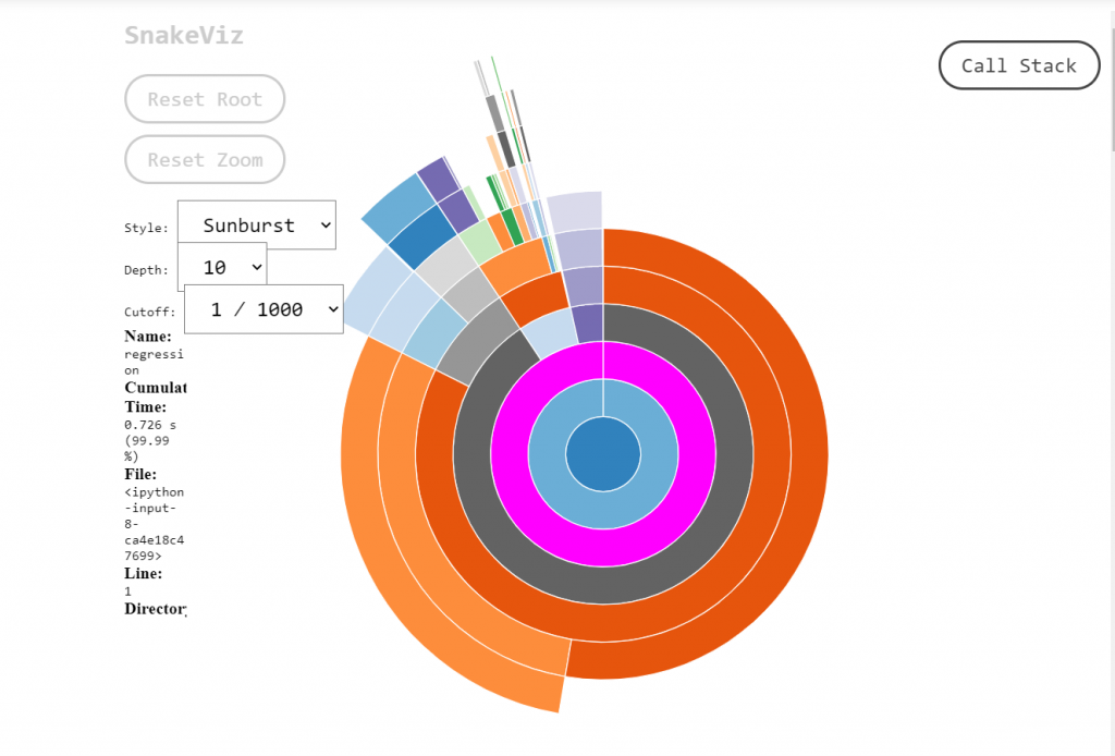
7. Profiling: Neresi Yavaş?

Kodunuzu optimize etmeden önce neresinin yavaş olduğunu bulmalısınız. prun veya kütüphaneleri kullanabilirsiniz ama Pandas için en kolayı pandas-profiling (yeni adıyla ydata-profiling) veya basitçe %timeit magic komutunu (Jupyter’da) kullanmaktır.

# Jupyter Notebook hücresinde
%timeit df['close'] - df['open']

Bu size o satırın kaç milisaniye sürdüğünü söyler. Tahmin yürütmeyin, ölçüm yapın. Bazen yavaşlık disk okumadadır, bazen hesaplamada. Sorunu bilmeden onaramazsınız.

8. Sınırları Zorlamak: Numba ve Polars

Vektörizasyon bile yetmiyorsa (örneğin karmaşık döngüler zorunluysa), Numba kullanın. @jit dekoratörü ile Python fonksiyonunu makine koduna (LLVM) derler. C++ hızına ulaşırsınız.

from numba import jit

@jit(nopython=True)
def calculate_complex_indicator(prices):
    # Saf Python döngüleri burada IŞIK HIZINDA çalışır
    result = []
    for price in prices:
        # Karmaşık matematik...
        result.append(price * 1.5)
    return result

Eğer veri RAM’e sığmıyorsa veya Pandas hantal kalıyorsa, Polars kütüphanesine geçin. Rust ile yazılmıştır, Lazy Evaluation kullanır ve Pandas’tan çok daha hızlıdır. Pandas 2.0 (PyArrow backend) ile hızlandı ama Polars hala kraldır.

Sonuç

Pandas yavaş değildir, onu yavaş kullanan bizleriz. Python’un esnekliği bazen “tembel” kod yazmamıza neden olabilir. Ancak büyük veri setlerinde bu tembelliğin bedeli ağır olur. Vektörizasyon mantığını kavradığınızda, Matrix filmindeki Neo gibi dünyayı 0 ve 1’ler (Matrixler) olarak görmeye başlarsınız.

Proje Önerileri:

• Eski projelerinizi açın ve iterrows() içeren yerleri temizleyin.
• CSV yerine Parquet formatına geçin.
• Zaman serisi analizlerinde rolling ve shift fonksiyonlarını aktif kullanın.
• Bellek tasarrufu için veri tiplerini (astype) manuel belirtin.
• Kodunuzu daha okunabilir kılmak için Method Chaining stilini deneyin.

Döngülerden kurtulun, veri tiplerine dikkat edin ve modern dosya formatlarını kullanın. Özellikle finansal veriler, zaman serileri ve büyük log dosyalarıyla çalışıyorsanız, bu teknikler bir tercih değil zorunluluktur. Şimdi gidin ve o for döngülerini kodunuzdan silin.